Are you tired of scrolling through endless rows of data in Excel, trying to find the information you need? Look no further! In this article, we will show you simple techniques for data organization that will make your life much easier.
With the ability to freeze multiple rows in Excel, you can keep important information in sight at all times, without losing track of your place. We will guide you through the process of using the Freeze Panes feature and demonstrate how to freeze multiple rows for effortless data navigation.
Additionally, we will introduce you to the Split Panes function, which allows for enhanced data viewing. Get ready to become an Excel pro as we share tips and tricks for efficient data organization in this comprehensive guide.
Say goodbye to the days of endless scrolling and hello to a more organized and productive Excel experience!
Understanding the Importance of Data Organization in Excel
You need to understand the importance of data organization in Excel, or else you’ll be overwhelmed and frustrated by the chaos of your spreadsheets.
When your data is scattered all over the place, it becomes difficult to find what you need quickly and efficiently. This can lead to errors, wasted time, and missed opportunities.
By organizing your data, you can easily locate and analyze information, making your work much more productive. Excel provides various tools and techniques to help you organize your data effectively.
You can use features like freezing rows to keep important information visible as you scroll through your spreadsheet.
By taking the time to organize your data, you’ll save yourself from the headache of searching for information and improve your overall efficiency in Excel.
Using the Freeze Panes Feature in Excel
To easily keep track of your spreadsheet, just freeze certain sections using Excel’s handy feature. Freezing panes allows you to lock rows or columns in place, making it easier to navigate through large amounts of data.
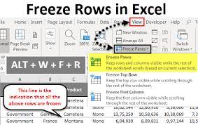
By freezing multiple rows, you can ensure that important headers or labels are always visible, even when scrolling down. To do this, simply select the row below the section you want to freeze, go to the View tab, and click on Freeze Panes. This will keep the selected row and all rows above it visible at all times.
By utilizing this feature, you can effortlessly organize your data and improve your productivity when working with large spreadsheets.
Freezing Multiple Rows for Easy Data Navigation
Enhance your productivity by effortlessly organizing your spreadsheet using Excel’s convenient feature that keeps important information visible as you navigate through large amounts of data.
Freezing multiple rows in Excel is a simple technique that allows you to lock specific rows at the top of your worksheet, making it easier to reference important data while scrolling through your spreadsheet.
To freeze multiple rows, select the row below the last row you want to freeze. Then, go to the View tab and click on the Freeze Panes option. From the drop-down menu, choose the ‘Freeze Panes’ option.
Now, when you scroll through your spreadsheet, the frozen rows will remain visible at the top, ensuring easy access to the essential information you need.
Utilizing Split Panes for Enhanced Data Viewing
When using split panes in Excel, you can effortlessly view different sections of your data side by side. This allows for a more comprehensive analysis of your spreadsheet. To utilize split panes, first select the cell where you want the split to occur. Then, go to the ‘View’ tab in the ribbon and click on ‘Split’.
This will create a vertical or horizontal split, depending on your selection. You can adjust the split by dragging the split bar to the desired position. With split panes, you can compare data from different parts of your spreadsheet without constantly scrolling back and forth.
This feature is particularly helpful when dealing with large datasets or when you need to compare data from different categories.
Tips and Tricks for Efficient Data Organization in Excel
One effective way to streamline your Excel workflow is by implementing smart strategies for efficiently organizing your information. When working with large datasets, it’s essential to have a clear structure that allows for easy navigation and analysis.
One helpful tip is to use color-coding to categorize different types of data. For example, you can assign a specific color to sales data and another color to expenses. This visual distinction makes it easier to quickly identify and analyze specific information.
Another useful trick is to use named ranges for your data. By assigning a name to a range of cells, you can easily refer to it in formulas and avoid the hassle of manually selecting cells each time.
These techniques will help you stay organized and save time when working with Excel.
Frequently Asked Questions
How do I freeze multiple rows in Excel using a keyboard shortcut?
To freeze multiple rows in Excel using a keyboard shortcut, select the row below where you want to freeze and press “Ctrl + Shift + 1”. This will keep those rows visible when scrolling through your spreadsheet.
Can I freeze multiple rows and columns simultaneously in Excel?
Yes, you can freeze multiple rows and columns simultaneously in Excel. To do this, select the cell below the rows and to the right of the columns you want to freeze, then go to the View tab and click on Freeze Panes.
Is it possible to freeze specific rows in Excel while keeping others unfrozen?
Yes, you can freeze specific rows in Excel while keeping others unfrozen. This allows you to easily navigate through your data. Simply select the row below the ones you want to freeze and go to the View tab, then click on Freeze Panes.
Are there any limitations to freezing multiple rows in Excel?
Yes, there are limitations to freezing multiple rows in Excel. You can only freeze rows that are visible on the screen, and it may affect the visibility of other data.
Can I freeze multiple rows in Excel without using the Freeze Panes feature?
Yes, you can freeze multiple rows in Excel without using the freeze panes feature. Simply select the row below the rows you want to freeze, then go to the View tab and click on Freeze Top Row.
Conclusion
In conclusion, organizing your data in Excel is crucial for efficient data management. By utilizing the Freeze Panes feature, you can easily freeze multiple rows to navigate through large datasets effortlessly.
Additionally, the Split Panes feature allows for enhanced data viewing, making it easier to compare and analyze information.
Remember to implement helpful tips and tricks, such as using color coding and sorting functions, to further optimize your data organization in Excel.
With these techniques, you can streamline your workflow and make the most out of your data.